The AGMS or tug-of-war sketch was proposed by Alon et al. based on the idea of using the square of the rope displacement on a tug-of-war game as an estimation of the skew of the distribution.

To do so, elements are assigned to a random team by using a $\pm1$ 4-wise random variable ($\xi$) and the rope displacement can be computed in the following way: $x = \sum\limits_{\forall e \in R}\xi(e)$.

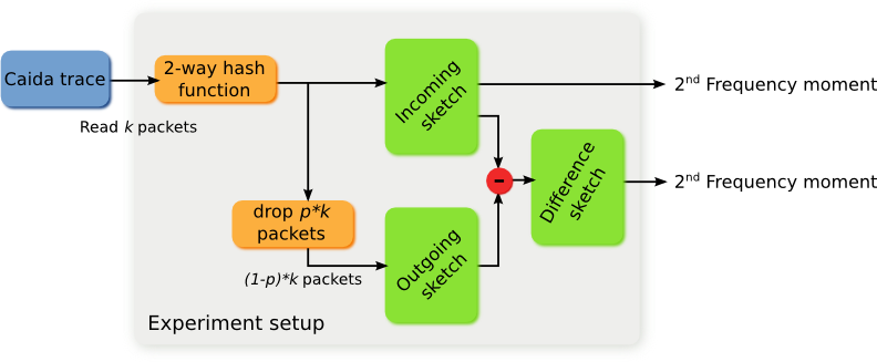
Statistically, the rope displacement measures the difference between the two teams and the expected value of its square matches the 2^nd frequency moment, with certain variance. To reduce this variance, Alon et al. propose combining several estimations as shown in the figure below.

Each counter on the AGMS sketch represents a tug-of-ware game and when a new element arrives every counter is updated ($x[i]=x[i]+\xi_i(e)$) using independent $\xi$ variables. Every row of the sketch, with $n$ counters, represents a basic estimator and gives the following estimation for the 2^nd frequency moment: $\frac{1}{n}\sum_1^n x[i]^2$. And then, the basic estimations are again combined using the median to increase the probabilistic confidence of the estimation:

$$\widehat{F_2}=median_{1 \le k \le m}(\frac{1}{n}\sum_1^n x_k[i]^2)$$

The resulting sketch is a matrix of $m \times n$ counters each with a $\xi$ random function associated.

The quality of the estimation is given by the following inequality (see Alon's paper for the details):

$$Prob(|\widehat{F_2} - F_2| \le \frac{4}{\sqrt{n}} \times F_2) \ge 1 - 2^{-m/2}$$

So the columns of the sketch (counters per basic estimator) determine the bounds of the error while the rows (number of basic estimators) affect the probabilistic confidence of the estimation. The variance of the basic estimator from Rusu's paper is:

$$Var[\widehat{F_2}] = 2 \times \frac{\left( F_2^2 - F_4 \right)}{n}$$

Where $F_4 = \sum\limits_{\forall e_i \in S} f_i^4$ is the 4^th frequency moment of the difference between traffic streams. So we can expect less precise estimations when the difference between two traffic streams is bigger than for pretty similar streams.

Evaluation

Our goal is to understand how the AGMS sketch performs on the traffic validation task. First we need to understand the difference between the theoretical bounds and empirical expectations: the bounds just set a limit on the quality of the estimation, but they are not necessarily a good estimation for the expected error range (as we will see). Also, we introduce a 2-way hash function in the process to reduce the input space; how does that affect the sketch's accuracy? Finally, for traffic validation we do not estimate the 2^nd frequency moment but a proportion; are the trends of the theoretical bounds also valid for that estimation?

Theoretical bounds

We mentioned before that the theoretical bounds for the AGMS sketch are:

$$Prob(|\widehat{F_2} - F_2| \le \frac{4}{\sqrt{n}} \times F_2) \ge 1 - 2^{-m/2}$$

To study how close this bound comes to experimental results we have done some experiments varying each of the parameters separately.

The general setup was the following: to create the incoming sketch we used a CAIDA trace, read 100 packets and filled the missing bits randomly. Then a 2-way hash function was applied and the resulting element sketched. On the other hand, the outgoing sketch was produced by dropping a percentage of the incoming packets.

Columns experiment

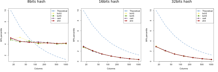
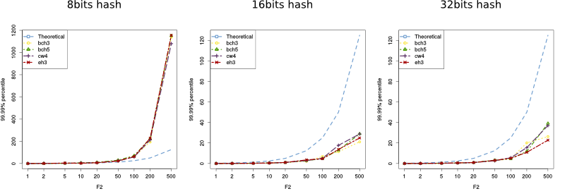
To study the effect of the number of columns we sketched 100 packets and dropped the 10% (10 packets). The size of the sketch was 14 rows and different values for the columns (16, 32, 64, 128, 256, 512 and 1024). Additionally, to see the effect of the 2-way hash function, we have tried with hashes of different lengths (8, 16, 32, 64 and 128) and also we have used different random generators (BCH3, BCH5, EH3 and CW4, see Rusu's paper for more details).

Given those parameters, the expected theoretical bound is:

$$Prob(|\widehat{F_2} - F_2| \le \frac{4}{\sqrt{n}} \times 10) \ge 1 - 2^{-14/2} = 0.996$$

The results are shown in the figure below for different lengths of the 2-way hash function. As we can see, for hashes of length 8, the probability of collision is too big, so the theoretical bounds do not fit within the theoretical limits, but for the rest are way below it. Results for bigger hash sizes were the same as for 16 or 32 bits.

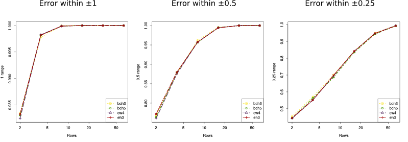
Rows experiment

Regarding the number of rows, we did a similar set of experiments: each incoming sketch has 100 packets and 10% of them were dropped to create the outgoing sketch; but this time we fixed the number of columns (512) and varied the number of rows (between 2, 4, 8, 16, 32 and 64).

In this case the theoretical bound on the error is:

$$Prob(|\widehat{F_2} - F_2| \le \frac{4}{\sqrt{516}} \times 10) = Prob(|\widehat{F_2} - F_2| \le 1.76) \ge 1 - 2^{-m/2}$$

The results are shown in the figures below where the 'y' axis represents the empirical probability of the error being smaller than 1.76. Again, we can see that all, but the 8 bits long hash, perform within the bounds and way better than they predict.

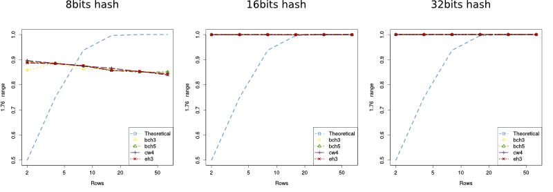
On the next figure we show the empirical probability for other ranges (only for the case of hashes of 32 bits) and as we can see, for 512 columns, keeping the error within a reasonable margin does not require many rows.

$F_2$ experiment (ongoing work)

Finally, we did a set of experiments modifying the value of $F_2$ to see how it affected the error. In this case, to have a wider number of values we sketched 1000 packets on the incoming sketch and used different drop probabilities (0.001, 0.002, 0.005, 0.01, 0.02, 0.05, 0.1, 0.2 and 0.5), which in return gave us different $F_2$ values (1, 2, 5, 10, 20, 50, 100, 200 and 500). On the other hand, the size of the sketch is fixed: 256 columns by 32 rows, giving us the following bounds:

$$Prob(|\widehat{F_2} - F_2| \le \frac{4}{\sqrt{256}} \times F_2) = Prob(|\widehat{F_2} - F_2| \le 0.25 \times F_2) \ge 1 - 2^{-32/2} = 0.9999847 $$

We see again the same results as before: as long as the hash is bigger than 16 bits, the sketches perform way better than expected.

Error distribution for the absolute error

The goal of the next set of experiments was to learn and characterize the distribution of the absolute error for the 2^nd frequency moment estimation. As before, we considered the clumns, rows and $F_2$ separately, but given that the hash length (for values higher than 16) and the random generator did not seem to affect much the sketch's accuracy, we only used the EH3 random generator and the 32 bits long hash.

Columns experiment

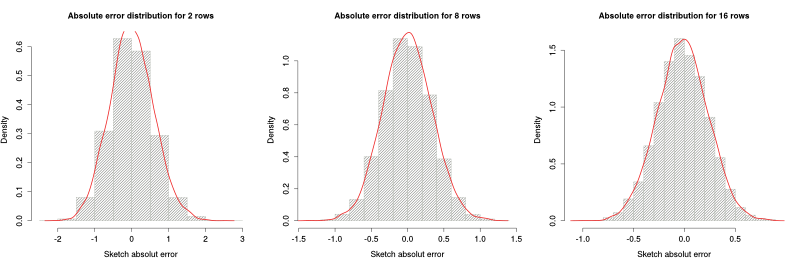
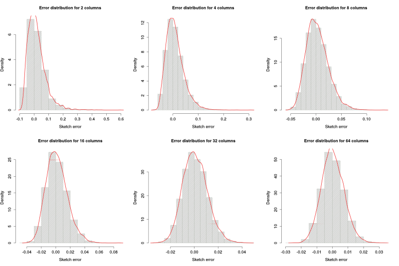
Our goal on this experiment was to see if the distribution of the error can be estimated as a Gaussian random variable and , if so, what is the relation between the number of columns and $\sigma$.

The parameters were very similar to the previous ones: 100 packets per incoming sketch, 10% packets dropped, 16 rows and a varying number of columns (2,4, 8, 16, 32, 64, 128, 256, 512 and 1024).

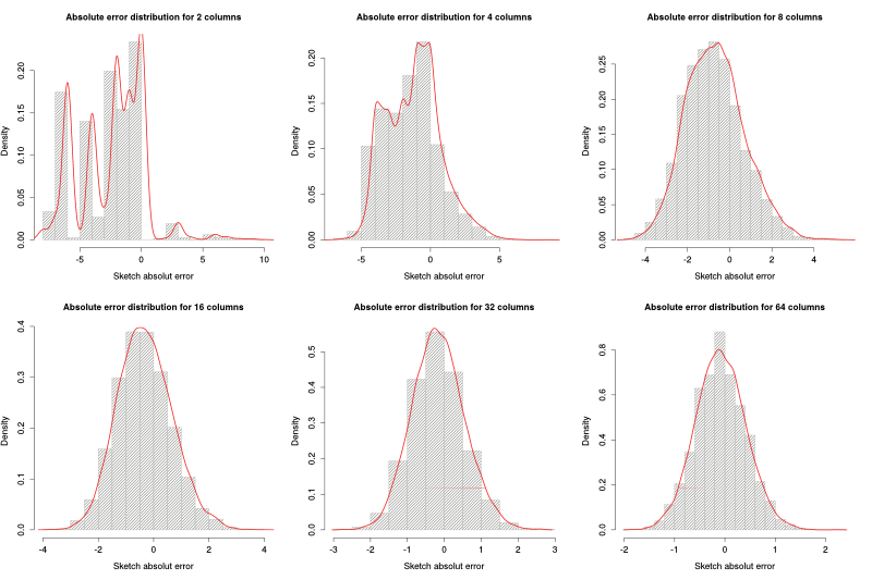
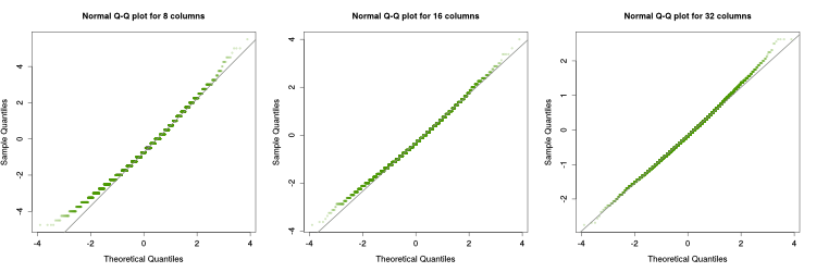
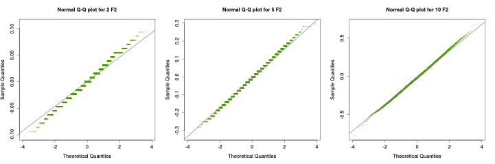
The figure above shows the histogram and estimated density function for different number of columns. As we can see, as the number of columns increases, the error distribution comes closer to a Gaussian distribution. Below we can see the Q-Q plots for 8, 16 and 32 columns: for more than 16 columns, the distribution of the error is pretty Gaussian.

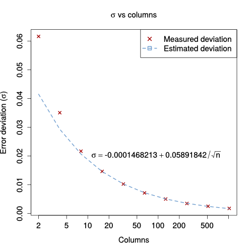
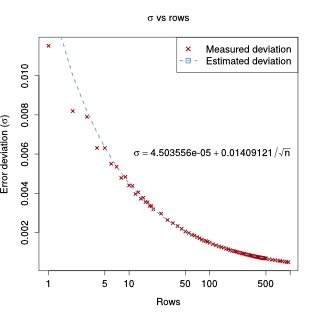
We know that the distribution of the error is centered at 0, but we still need to know which is the value of $\sigma$. Using the standard deviation obtained on the experiments and doing a linear regression over the $z=\frac{1}{\sqrt{n}}$ we obtain the following formula:

$$ 0.0055 + 3.95 \times \frac{1}{\sqrt{n}} \approx 4 \times \frac{1}{\sqrt{n}}$$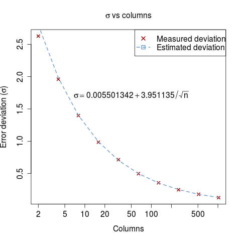

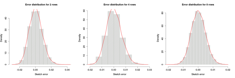
Rows experiment

Regarding the rows, the setup was similar, only this time the sketch had 256 columns and a wide range of values between 1 to 1000 for the number of rows. As the figures below show, the distribution of the error is already Gaussian even for low number of rows. We believe this is due to the high number of columns and the fact that columns and rows have a really similar role in the AGMS sketch; so in the end what needs to be big enough is the product $n \times m$.

The relation between the standard deviation and the number of rows is again proportional to $\frac{1}{\sqrt{m}}$ (but the fit is not as close as for the number of columns):

$$ 0.0150 + 0.89 \times \frac{1}{\sqrt{m}}$$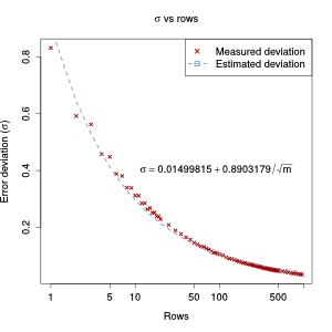

F2 experiment

Finally, for measuring how the error varies with columns $F_2$, we used a 256 columns by 32 rows sketch and different drop probabilities over 1000 packets. Again, the distribution is more Gaussian for higher values of $F_2$ and the error for the estimation of a 10 or higher packets' difference can be approximated as Gaussian.

In this case, the error's standard deviation increases linearly with the 2^nd frequency moment:

$$ -0.019 + 0.02 \times F_2$$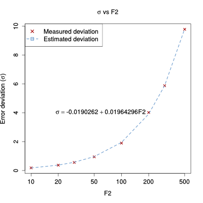

Error distribution for the drop percentage estimation

However, for Traffic Validation we do not care as much for the number of packets lost but for the proportion of packets lost (or corrupted), which will be estimated as:

$$\widehat{dp} = \frac{F_2(Sketch_{incoming} - Sketch_{outgoing})}{F_2(Sketch_{incoming})}$$

The goal of the following analysis is to see if the estimation of the percentage is accurate and how does the number of rows, columns and packets affect this accuracy. The figures and analysis was done using the data of the previous experiments, so please refer to them for the values of the different parameters.

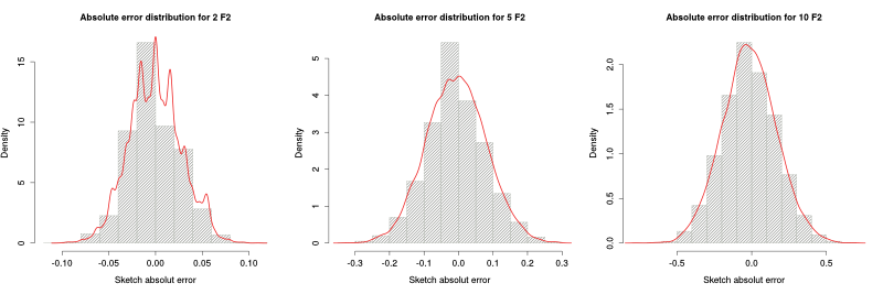
Columns experiment

As we can see in the figure below, the error for the packet percentage estimation has a long right tail for smaller number of columns, but tends to Gaussian for higher values

The quality of the prediction drops compared to the error in estimating the 2^nd frequency moment (e.g. obtaining a deviation for the error below 10% of the value requires 32 columns instead of 16 for $F_2$); which was expected since now the sketch has to predict two different $F_2$ (for the incoming sketch and difference sketch) instead of just one. The relation between the standard deviation and the number of columns (when the number of columns is high enough) is still proportional to $\frac{1}{\sqrt{n}}$: $$ \sigma = 0.0589 \times \frac{1}{\sqrt{n}}$$

Rows experiment

Similarly, higher rows provide a more Gaussian distribution of the error, but (again because of the high number of columns) not as much as the number of columns on the previous experiment.

The deviation of the error, too, can be estimated as a function of $\frac{1}{\sqrt{m}}$:

$$ \sigma = 0.014 \times \frac{1}{\sqrt{m}}$$

But again, in relative terms, more rows are required for similar performance, when compared with the estimation of the number of dropped packets instead of its ratio.

Difference Sketch's $F_2$ experiment

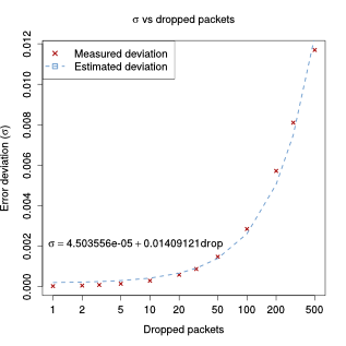
On the case of the ratio between dropped packets and input packets, there are two 2^nd frequency moments to take into account. This first experiment takes a look at the effect of the dropped packets' $F_2$. To do so, we used a sketch of 256 columns by 32 rows and 1000 packets for the incoming sketch. Different drop probabilities gave us different number of dropped packets ranging from 1 to 500.

The histograms below show that in this case the distribution has on every scenario a smal left tail. We beliefe this was due to the high number of packets in the incoming sketch.

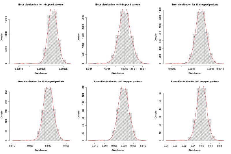
Even though in this case we cannot fairly represent the distribution of the error with a Gaussian distribution, we decided to use the standard deviation as a measure of the spread of the error; and consequently a measure of the quality of the prediction. As the figure below shows, $\sigma$ is proportional to the number of packets dropped:

$$\sigma = 0.014 \times dropped\_packets$$